Capacity

Design gross output (MWe)

The power cycle's design output, not accounting for parasitic losses. SAM uses this value to size system components, such as the solar field area when you use the solar multiple to specify the solar field size.

Estimated gross to net conversion factor

An estimate of the ratio of the electric energy delivered to the grid to the power cycle's gross output. SAM uses the factor to calculate the system's nameplate capacity for capacity-related calculations.

Estimated net output at design (MWe)

The power cycle's nominal capacity, calculated as the product of the design gross output and estimated gross to net conversion factor. SAM uses this value for capacity-related calculations, including the estimated total cost per net capacity value on the Installation Costs page, capacity-based incentives on the Cash Incentives page, and the capacity factor reported in the results.

Estimated Net Output at Design (MWe) = Design Gross Output (MWe) × Estimated Gross to Net Conversion Factor

System Availability

System availability losses are reductions in the system's output due to operational requirements such as maintenance down time or other situations that prevent the system from operating as designed.

Notes.
 
To model curtailment, or forced outages or reduction in power output required by the grid operator, use the inputs on the Grid Limits page. The Grid Limits page is not available for all performance models.
 
For the PV Battery model, battery dispatch is affected by the system availability losses. For the PVWatts Battery, Custom Generation Profile - Battery, and Standalone Battery battery dispatch ignores the system availability losses.

To edit the system availability losses, click Edit losses.

The Edit Losses window allows you to define loss factors as follows:

•Constant loss is a single loss factor that applies to the system's entire output. You can use this to model an availability factor.

•Time series  losses apply to specific time steps.

SAM reduces the system's output in each time step by the loss percentage that you specify for that time step. For a given time step, a loss of zero would result in no adjustment. A loss of 5% would reduce the output by 5%, and a loss of -5% would increase the output value by 5%.

Conversion

Note. The generic solar system model's steam turbine model is based on the empirical parabolic trough model's power block model. For a description of how SAM uses the part-load and temperature adjustment coefficients, see Power Block Simulation Calculations.

Reference conversion efficiency

Total thermal to electric efficiency of the reference turbine at design. Used to calculate the design turbine thermal input and required solar field aperture area.

Max over design operation

The turbine's maximum output expressed as a fraction of the design turbine thermal input. Used by the dispatch module to set the power block thermal input limits. In cases where the normalized thermal power delivered to the power block by the solar field exceeds this fraction, the field will dump excess energy.

Minimum load

The turbine's minimum load expressed as a fraction of the design turbine thermal input. Used by the dispatch module to set the power block thermal input limits. In cases where the solar field, thermal storage, and/or fossil backup system are unable to produce enough energy to meet this fractional requirement, the power cycle will not produce electricity.

Power cycle startup energy

Hours of equivalent full-load operation of the power cycle required to bring the system to operating temperature after a period of non-operation. Used by the dispatch module to calculate the required start-up energy.

Boiler LHV Efficiency

The back-up boiler's lower heating value efficiency. Used by the power block module to calculate the quantity of gas required by the back-up boiler.

Power cycle design ambient temperature

The ambient temperature at which the power cycle conversion efficiency is equal to the reference conversion efficiency. The temperature corresponds to either the wet-bulb or dry-bulb temperature, depending on the value selected by the user in the Temperature correction mode list. The temperature is used in the Temperature adjustment polynomial in the Parasitics group on the Power Block page to determine cycle conversion efficiency.

Part load efficiency adjustment

Coefficients for the turbine thermal-to-electric efficiency polynomial equation. This polynomial is used to adjust the cycle conversion efficiency as the thermal load into the power cycle varies from its design-point value. The resulting value from the evaluated polynomial multiplies the reference conversion efficiency, where the polynomial is formulated as follows:

Temperature efficiency adjustment

Factors for polynomial equation adjusting power cycle efficiency based on the difference between the power cycle design temperature and ambient temperature (either wet bulb or dry bulb temperature from the weather file, depending on the option you choose for Temperature Correction Mode.) The polynomial is formulated as follows:

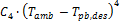
where Tamb is the wet or dry bulb temperature, depending on the Temperature Correction Mode selection.

The power cycle conversion efficiency is calculated as the product of the Reference conversion efficiency and the summation of the two polynomial efficiency adjustment terms.

Temperature Correction Mode

In the dry bulb mode, SAM calculates a temperature correction factor to account for cooling tower losses based on the ambient temperature from the weather data set. In wet bulb mode, SAM calculates the wet bulb temperature from the ambient temperature and relative humidity from the weather data.

Parasitics

Fixed parasitic load (MWe/MWcap)

A fixed hourly loss calculated as a fraction of the power block nameplate capacity.

Production based parasitic (MWe/MWe)

A variable hourly loss calculated as a fraction of the system's hourly electrical output. The total production-based parasitic is evaluated as follows:

where Fpar,prod,ref is the production based parasitic factor, Fpar,load is the load-based parasitic adjustment factor (defined below), and Fpar,temp is the temperature-based parasitic adjustment factor (also defined below), and Fpar,DNI is the solar resource-based parasitic adjustment factor (also defined below).

Part load adjustment

Coefficients for a polynomial that adjusts the parasitic consumption as a function of power cycle gross power output. The result of the polynomial is denoted as Fpar,load in the Production based parasitic description above.

Temperature adjustment

Coefficients for a polynomial that adjusts the parasitic consumption as a function of the difference between ambient temperature and the reference power cycle ambient temperature. The result of the polynomial is denoted as Fpar,temp in the Production based parasitic description above.

DNI adjustment

Coefficients for a polynimal that adjusts the parasitic consumption as a function of the solar resource value. The result of the polynomial is denoted as F_(par,DNI) in the Production based parasitic description above.