Solar Field Optical Efficiency Data

The solar position table option allows you to specify optical efficiency of the solar field as a function of solar azimuth and zenith angles. SAM uses a solar azimuth angle convention where true North is equal to -180/+180° and South equals 0°. The solar zenith angle is zero when the sun is directly overhead and 90° when the sun is at the horizon.

The solar position may contain any number of rows and columns, but should contain enough information to fully define the performance of the solar field at all sun positions for which the field will operate. The table must contain more than one row and column.

SAM uses linear interpolation to estimate efficiency values for solar positions between those specified on the table.

Import

Import a table from a text or data file. The file can contain values separated by comma, space, or tab characters, but must be formatted according to the following rules:

•The first row in the file specifies the angles for the solar azimuth (for the Solar position table) or collector transversal incidence (for the Collector incidence angle table). The first entry of this row should be blank.

•Each additional row specifies optical efficiency for a specific zenith angle (for the Solar position table) or longitudinal incidence angle (for the Collector incidence angle table). The first entry of the row must be the zenith or longitudinal incidence angle corresponding to the optical efficiency entries in that row.

•The rows of the table should be sorted according to zenith/longitudinal incidence angle from lowest to highest.

An example tab-delimited table is as follows, where numbers in bold correspond to the solar zenith (row headers) and azimuth (column headers) angles:

 -180        -90        0        90        180

0        1.0        1.0        1.0        1.0        1.0

30        0.95        0.98        0.99        0.98        0.95

60        0.60        0.70        0.75        0.70        0.60

90        0.0        0.0        0.0        0.0        0.0

Note that SAM automatically sizes the table on the Collector and Receiver page to match the size of the array that is being imported.

Export

Export the optical efficiency table on the Collector and Receiver page to a text file.

Copy

Copy the optical efficiency table on the Collector and Receiver page to the clipboard for transfer to an optical efficiency table in another case or to other text applications.

Paste

Paste an optical efficiency table from another SAM case or from a text file into the active case.

Rows

Specify the number of desired rows in the table.

Cols

Specify the number of desired columns in the table.

Interpolate table

Choose this option if you want SAM to use interpolation to calculate radiation values for points between those included in the table.

Irradiation basis

Determines the column of data that SAM reads from the weather file.

Unsorted data table mode

This option allows you to specify the solar field efficiency using a table of Sun Azimuth-Zenith pairs. SAM uses the Gauss-Markov method to interpolate efficiency values over the full range of sun positions.

Design Point Parameters

Solar Multiple

The field aperture area expressed as a multiple of the aperture area required to operate the power cycle at its design capacity. See Sizing the Solar Field for details.

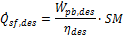
Solar field design output (MWt)

The thermal energy delivered by the solar field under design conditions at the given solar multiple. This value is calculated in the interface as the function of the solar multiple, the Reference conversion efficiency on the Power Block page, and the Design gross output on the Power Block page, as follows:

Ambient temp at design (°C)

The design point ambient temperature (dry-bulb), used to calculate solar field thermal efficiency and the aperture area required to drive the power cycle at its design capacity.

Solar resource at design (W/m²)

The design point direct normal radiation value, used in solar multiple mode to calculate the aperture area required to drive the power cycle at its design capacity.

Stow angle (degrees)

The collector angle during the hour of stow. A stow angle of zero for a northern latitude is vertical facing east, and 180 degrees is vertical facing west. Default is 170 degrees.

Deploy angle (degrees)

The collector angle during the hour of deployment. A deploy angle of zero for a northern latitude is vertical facing due east. Default is 10 degrees.

Estimated Solar Field Area (m²)

The total solar energy collection area of the solar field in square meters.

Estimated Solar Field Area = ( Solar Field Design Output + Thermal Loss at Design )
                                      / Total Optical Efficiency × 1,000,000
                                      / Solar Resource at Design

 

Note. This estimate of the solar field area is different from the design solar field area used in calculations for the simulation. For the simulation, SAM calculates the design solar field area from the optical efficiency at noon on the summer solstice (June 21).

Efficiency Derates

Peak optical efficiency

The maximum value of the optical efficiency values in the Solar Field Optical Efficiency Data table.

Cleanliness factor

A derating factor to account for optical losses by soiling on the mirror surface or other losses.

General optical derate

Accounts for reduction in absorbed radiation caused by general optical errors or other unaccounted error sources.

Total optical efficiency

The product of the three optical efficiency factors.

Solar Field Availability

The Edit Losses window allows you to specify fixed, hourly, and/or hourly losses within custom periods. Losses effectively reduce (or increase) the optical efficiency of the solar field during the affected hour(s).

Generalized Thermal Losses

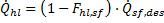
Reference thermal loss fraction

The fraction of thermal power generated by the solar field that is lost to thermal losses at design. The heat loss calculation during the annual hourly performance run multiplies this value by the resulting values of the heat loss correction polynomials to obtain the total solar field thermal efficiency. The thermal losses from the solar field are evaluated according to the following relationship, where the various Fhl coefficients are evaluated according to the descriptions provided below.

Irradiation thermal loss adjustment

This polynomial adjusts the thermal loss fraction in the solar field as a function of the solar irradiation available during the current time step of the performance simulation. The polynomial is evaluated to determine the sensitivity of thermal losses to irradiation as follows:

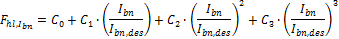
where Ibn is the solar irradiation during the current time step and Ibn,des is the design-point solar irradiation from the Solar resource at design input on the Solar Field page.

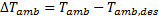
Ambient temp thermal loss adjustment

This polynomial adjusts the thermal loss fraction in the solar field as a function of the ambient dry-bulb temperature in degrees Celsius. The Reference thermal loss fraction is multiplied by the result of the following polynomial:

where

or the ambient temperature for the current time step of the simulation minus the ambient dry-bulb temperature at design.

Wind speed thermal loss adjustment

This polynomial adjusts the thermal loss fraction in the solar field as a function of the wind speed during the current time step of the performance simulation. The result of the evaluated wind speed adjustment polynomial multiplies the Reference thermal loss fraction and other correction polynomials to determine the total solar field efficiency. The polynomial is evaluated as follows:

where

Thermal loss at design

The calculated thermal losses at design conditions, equal to the product of the Reference thermal loss fraction and the Solar field design output. SAM calculates actual thermal losses during simulation runs using on the design-point thermal losses and the results of the thermal loss correction polynomials described above. The design thermal losses are used to size the aperture area of the solar field that is required to drive the power cycle.