The System Design page shows inputs for design point parameters that determine the system's nameplate capacity. Use the System Design inputs to define the nominal ratings of the system, and then specify details for each part of the system on the appropriate input pages.
Note. All of the system design inputs are nominal values, or values at the system's design point. SAM calculates actual values during simulation and reports them in the results.
Solar Field
The solar field design parameters determine the size of the solar field. See the Solar Field, Collectors (SCAs), and Receivers (HCEs) pages to set detailed parameters for the field.
Option 1 and Option 2
For Option 1 (solar multiple mode), SAM calculates the total required aperture and number of loops based on the value you enter for the solar multiple.
For option 2 (field aperture mode), SAM calculates the solar multiple based on the field aperture value you enter. Note that SAM does not use the value that appears dimmed for the inactive option. See Solar Multiple for details.
Solar Multiple
The field aperture area expressed as a multiple of the aperture area required to operate the power cycle at its design capacity. See Solar Multiple for details.
Field Aperture (m²)
The total solar energy collection area of the solar field in square meters. Note that this is less than the total mirror surface area.
Note. For simulations, SAM uses the Actual Solar Multiple and Total Aperture Reflective Area values shown under Solar Field Design Point on the Solar Field page. The calculated value of the inactive option may differ from the value you see on the System Design page.
Design point DNI (W/m²)
The design point direct normal radiation value, used in solar multiple mode to calculate the aperture area required to drive the power cycle at its design capacity. Also used to calculate the design mass flow rate of the heat transfer fluid for header pipe sizing.
Field thermal power, MWt
The field thermal power output at design.
Field Thermal Power (MWt) = Solar Multiple × Cycle Thermal Power (MWt)
Loop inlet HTF temperature (ºC)
The temperature of HTF at the loop inlet under design conditions. The actual temperature during operation may differ from this value. SAM sets the power cycle's design outlet temperature equal to this value.
Loop outlet HTF temperature (ºC)
The temperature of the HTF at the outlet of the loop under design conditions. During operation, the actual value may differ from this set point. This value represents the target temperature for control of the HTF flow through the solar field and will be maintained when possible.
Number of loops
The number of loops in the field, equal to the solar multiple times the required number of loops at a solar multiple of 1.0. The required number of loops is rounded to the nearest integer to represent a realistic field layout.
Power Cycle
The power cycle design parameters determine the capacity of the power cycle, and the nameplate capacity of the system. See the Power Cycle page for more detailed power cycle options and detailed parameters.
Design turbine gross output (MWe)
The power cycle's design output, not accounting for parasitic losses. SAM uses this value to size system components, such as the solar field area when you use the solar multiple to specify the solar field size.
Estimated gross to net conversion factor
An estimate of the ratio of the electric energy delivered to the grid to the power cycle's gross output. SAM uses the factor to calculate the power cycle's nameplate capacity for capacity-related calculations, including the estimated total cost per net capacity value on the Installation Costs and Operating Costs pages capacity-based incentives on the Incentives page, and the capacity factor reported in the results.
Estimated net output at design (nameplate) (MWe)
The power cycle's nameplate capacity, calculated as the product of the design gross output and estimated gross to net conversion factor.
Estimated Net Output at Design (MWe) = Design Gross Output (MWe) × Estimated Gross to Net Conversion Factor
Cycle thermal efficiency
The thermal to electric conversion efficiency of the power cycle under design conditions
Cycle thermal power, MWt
The power cycle thermal power input at design.
Cycle Thermal Power, MWt = Design Turbine Gross Output (MWe) ÷ Cycle Thermal Efficiency
Thermal Storage
The thermal storage design parameters determine the size of the thermal energy storage system (TES). See the Thermal Storage page for detailed TES parameters.
Hours of storage at design point (hours)
The thermal storage capacity expressed in number of hours of thermal energy delivered at the design power cycle thermal power. The physical capacity is the number of hours of storage multiplied by the power cycle design thermal input. Used to calculate the thermal energy system's maximum storage capacity.
Solar Multiple
Sizing the solar field of a parabolic trough or linear Fresnel system in SAM involves determining the optimal solar field aperture area for a system at a given location. In general, increasing the solar field area increases the system's electric or thermal output, thereby reducing the project's levelized cost of energy. However, during times when there is enough solar resource, too large of a field will produce more thermal energy than the power cycle or heat sink and other system components can handle. Also, as the solar field size increases beyond a certain point, the higher installation and operating costs outweigh the benefit of the higher output.
An optimal solar field area should:
•Maximize the amount of time in a year that the field generates sufficient thermal energy to drive the power cycle or heat sink at its rated capacity.
•Minimize installation and operating costs.
•Use thermal energy storage and backup power equipment efficiently and cost effectively.
The problem of choosing an optimal solar field area involves analyzing the tradeoff between a larger solar field that maximizes the system's electrical output and project revenue, and a smaller field that minimizes installation and operating costs.
The levelized cost of energy (LCOE or LCOH) is a useful metric for optimizing the solar field size because it includes the amount of electricity or heat generated by the system, the project installation costs, and the cost of operating and maintaining the system over its life. Optimizing the solar field involves finding the solar field aperture area that results in the lowest LCOE or LCOH. For systems with thermal energy storage systems, the optimization involves finding the combination of field area and storage capacity that results in the lowest LCOE or LCOH.
Option 1 and Option 2
SAM's parabolic trough and linear Fresnel models provide two options for specifying the solar field aperture area on the System Design page:
•Option 1: You specify the solar field area as a multiple of the power cycle (design turbine gross output) or heat sink rated capacity (heat sink thermal power), and SAM calculates the solar field aperture area in square meters required to achieve the rated capacity.
•Option 2: You specify the aperture area in square meters independently of the power cycle or heat sink rated capacity.
If your analysis involves a known solar field area, you should use Option 2 to specify the solar field aperture area.
If your analysis involves optimizing the solar field area for a specific location, or choosing an optimal combination of solar field aperture area and thermal energy storage capacity, then you should choose Option 1, and follow the procedure described below to size the field.
Solar Multiple
Note. The description in this section refers to the power cycle of a system that generates electricity. For industrial process heat (IPH) systems, the same principles apply, but are determined by the heat sink capacity rather than the power cycle capacity.
The solar multiple makes it possible to represent the solar field aperture area as a multiple of the power cycle rated capacity. A solar multiple of one (SM=1) represents the solar field aperture area that, when exposed to solar radiation equal to the design point DNI (or irradiation at design), generates the quantity of thermal energy required to drive the power cycle at its rated capacity (design gross output), accounting for thermal and optical losses.
Because at any given location the number of hours in a year that the actual solar resource is equal to the design point DNI is likely to be small, a solar field with SM=1 will rarely drive the power cycle at its rated capacity. Increasing the solar multiple (SM>1) results in a solar field that operates at its design point for more hours of the year and generates more electricity.
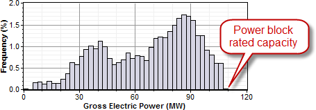
For example, consider a system with a power cycle design gross output rating of 111 MW and a solar multiple of one (SM=1) and no thermal storage. The following frequency distribution graph shows that the power cycle never generates electricity at its rated capacity, and generates less than 80% of its rated capacity for most of the time that it generates electricity:
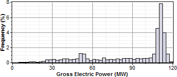
For the same system with a solar multiple chosen to minimize LCOE (in this example SM=1.5), the power cycle generates electricity at or slightly above its rated capacity almost 15% of the time:
Adding thermal storage to the system changes the optimal solar multiple, and increases the amount of time that the power cycle operates at its rated capacity. In this example, the optimal storage capacity (full load hours of TES) is 3 hours with SM=1.75, and the power cycle operates at or over its rated capacity over 20% of the time:
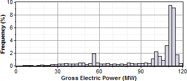
Note. For clarity, the frequency distribution graphs above exclude nighttime hours when the gross power output is zero.
Reference Weather Conditions for Field Sizing
The design weather conditions values are reference values that represent the solar resource at a given location for solar field sizing purposes. The field sizing equations require three reference condition variables:
•Ambient temperature
•Direct normal irradiance (DNI)
•Wind velocity
The values are necessary to establish the relationship between the field aperture area and power cycle rated capacity for solar multiple (SM) calculations.
Note. The design values are different from the data in the weather file. SAM uses the design values to size the solar field before running a simulation. During the simulation, SAM uses data from the weather file you choose on the Location and Resource page.
The reference ambient temperature and reference wind velocity variables are used to calculate the design heat losses, and do not have a significant effect on the solar field sizing calculations. Reasonable values for those two variables are the average annual measured ambient temperature and wind velocity at the project location. For the physical trough model, the reference temperature and wind speed values are hard-coded and cannot be changed. The linear Fresnel and generic solar system models allow you to specify the reference ambient temperature value, but not the wind speed. The empirical trough model allows you to specify both the reference ambient temperature and wind speed values.
The reference direct normal irradiance (DNI) value, on the other hand, does have a significant impact on the solar field size calculations. For example, a system with reference conditions of 25°C, 950 W/m2, and 5 m/s (ambient temperature, DNI, and wind speed, respectively), a solar multiple of 2, and a 100 MWe power cycle, requires a solar field area of 871,940 m2. The same system with reference DNI of 800 W/m2 requires a solar field area of 1,055,350 m2.
In general, the reference DNI value should be close to the maximum actual DNI on the field expected for the location. For systems with horizontal collectors and a field azimuth angle of zero in the Mohave Desert of the United States, we suggest a design irradiance value of 950 W/m2. For southern Spain, a value of 800 W/m2 is reasonable for similar systems. However, for best results, you should choose a value for your specific location using one of the methods described below.
Linear collectors (parabolic trough and linear Fresnel) typically track the sun by rotating on a single axis, which means that the direct solar radiation rarely (if ever) strikes the collector aperture at a normal angle. Consequently, the DNI incident on the solar field in any given hour will always be less than the DNI value in the resource data for that hour. The cosine-adjusted DNI value that SAM reports in simulation results is a measure of the incident DNI.
Using too low of a reference DNI value results in excessive "dumped" energy: Over the period of one year, the actual DNI from the weather data is frequently greater than the reference value. Therefore, the solar field sized for the low reference DNI value often produces more energy than required by the power cycle, and excess thermal energy is either dumped or put into storage. On the other hand, using too high of a reference DNI value results in an undersized solar field that produces sufficient thermal energy to drive the power cycle at its design point only during the few hours when the actual DNI is at or greater than the reference value.
To choose a reference DNI value:
1.Choose a weather file on the Location and Resource page.
2.For systems with storage, specify the storage capacity and maximum storage charge rate defined on the System Design page.
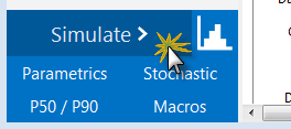
3.Click Simulate.
4.On the Results page, click Statistics.
5.Read the maximum annual value of Field collector DNI-cosine product (W/m2), and use this value for the reference DNI.
An alternative method is to choose a reference DNI value on the System Design page to minimize collector defocusing, to do this, try different values for Design point DNI on the System Design page until you find a value that minimizes the total Field fraction of focused SCAs output variable on the Statistics tab. You could also use parametric simulations to find the reference DNI value.